Quantitative Trading (2)

If you don’t get how industrialized trading works, your macro read is half-blind.

Who Is Actually Doing Quant in the Real World?

Globally, there are at least four layers of actors in the quant ecosystem. Outsiders often lump them together.

1. Systematic Asset Management Firms

First layer: systematic asset managers.

• AQR defines itself as a quant investor using a systematic and disciplined approach to long-term value and diversified strategies.

• Two Sigma emphasizes people, technology, data, and a scientific approach to finance.

• D.E. Shaw stresses its pioneering role in computational finance, its investment management, technology development, risk management, and deep talent base.

• Man Group states that it has a tradition of data-led quantitative investment, managing about $228.7 billion of AUM as of March 31, 2026, with over 600 quants and technologists.

• Winton explicitly calls itself a quantitative investment management firm, relying on original research, rigorous statistical analysis, and infrastructure to implement strategies across major liquid markets.

Taken together, these descriptions show that “global quant” is not a small circle of coders. It is industrial finance.

2. Market Makers and Proprietary Trading Firms

Second layer: market makers and proprietary trading firms.

• Citadel Securities, Optiver, and Virtu all use terms like market maker, liquidity, two-sided prices, and technology in their public descriptions.

• Jane Street emphasizes that it is a research-driven trading firm, and highlights capital, global reach, technology, expertise, and quantitative trading.

Their business models differ from classic hedge funds. They are not necessarily betting on long-run factors at all. They rely on:

• Quoting.

• Inventory management.

• Ultra-fast risk.

• Cross-market pricing.

• Execution infrastructure.

If systematic asset managers are “research–portfolio–capital machines,” market makers and prop firms are “microstructure–liquidity–execution machines.” Both are quant. They are not the same game.

3. Research, Data, and Infrastructure Providers

Third layer: research, data, and market infrastructure.

• Kenneth French’s Data Library provides the factor bedrock.

• Nasdaq sells alternative data.

• Coin Metrics handles on-chain and digital-asset datasets.

• Exchanges, clearinghouses, and regulators (CME, CSRC, ESMA, etc.) define microstructure, margin rules, and risk regimes.

Without this layer, quant cannot become an industrialized activity. Many people think the core of quant is “smart models.” In reality, a large share of an institutional shop’s productive capacity is in:

• Data cleaning.

• Point-in-time integrity.

• Storage.

• Permissions.

• Logging.

• Compliance.

• Risk.

4. Platforms, Open-Source Communities, and Toolchains

Fourth layer: platforms, open-source ecosystems, and toolchains that translate quantitative ideas into executable workflows.The

United States and international ecosystems are dominated by mature, broker-agnostic infrastructure. QuantConnect’s LEAN engine (US‑based, open‑source) allows strategy coding in Python or C# and backtesting across global equities, futures, forex, and crypto. Interactive Brokers (US) provides a battle-tested API that powers countless proprietary and retail systems, connecting to over 150 markets worldwide. MetaTrader’s Expert Advisors, though Russian in origin, remain a staple for retail forex and CFD traders internationally. Open‑source communities orbit these tools—Zipline (originally from Quantopian), Backtrader, and QuantLib—all contributing to a modular, transparent stack.

China’s ecosystem has evolved its own parallel infrastructure to serve A‑share markets and local regulatory demands. vn.py is an open‑source, production‑ready trading framework that wraps domestic broker APIs (CTP, XTP, etc.) and is widely used by small funds and independent traders. JoinQuant and RiceQuant offer cloud‑based research environments with Python APIs, curated data, and paper‑trading simulators integrated with Chinese brokers. MyQuant provides a low‑latency terminal and SDK for professional users. These platforms are not just translations of Western tools; they are purpose‑built for China’s market microstructure, settlement cycles, and data vendors.

All of these platforms, regardless of geography, reduce the barrier to entry:

• Some people use them for education.

• Some for research.

• Some connect to live capital.

• Some treat them as their primary workbench.

Their official descriptions almost always center on data, backtesting, simulation, APIs, and risk tools — not “guaranteed returns.” That alone tells you something:

Real quant platforms sell infrastructure, not performance promises.

A mature quant team is not held up by “one coder.” It usually includes:

• Quant researchers – signal generation, factor mining, literature review

• Quant traders/portfolio managers – execution logic, cost modeling, portfolio construction

• Developers – core framework, performance optimization, API integration

• Data engineers – cleaning, storing, and versioning petabytes of market and alternative data

• Execution engineers – smart order routing, broker connectivity, latency tuning

• Risk managers – real‑time exposure monitoring, stress testing, kill‑switch design

• Operations – reconciliation, settlement, position reporting

• Compliance – regulatory filings, pre‑trade checks, insider‑trading safeguards

Individuals can absolutely learn quant thinking. But installing Python, wiring up an API, and running a backtest does not mean you’ve cloned an institutional production pipeline. It means you’ve touched the outer layer of a far deeper, multi‑role, multi‑system machinery where infrastructure is necessary but never sufficient. The platform gives you the tools; the team, the process, and the edge give you the outcome.

---

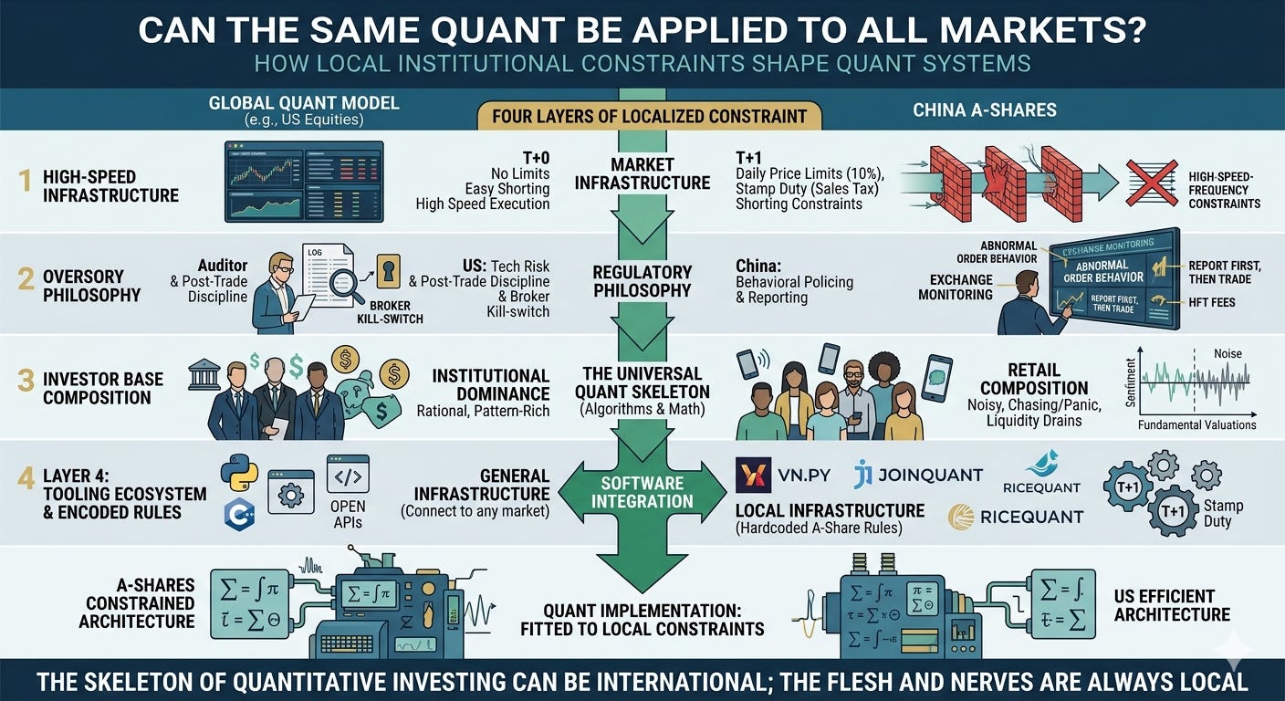
Can the same quant be applied to all markets?

Quant systems look very different from country to country, and the root cause is not algorithms or math. It’s four layers of institutional constraint that quietly shape everything.

1. The “Physical Rules” of Market Infrastructure

Start with the plumbing. China’s market design — T+1 stock settlement, daily price limits, stamp duty, and short-selling constraints — directly rewires holding periods, execution assumptions, and hedging design.

• T+1 settlement means shares bought today cannot be sold today.
  That instantly kills the US-style intraday equity scalping that many people imagine they can “copy” to A‑shares. If you want intraday turnover in China, you are pushed toward instruments that are effectively T+0: futures, some options, and convertibles.

• Price limits introduce a backtest landmine.
  On paper, your model might happily buy at the limit up or sell at the limit down. In reality, you may sit in the queue all day and never get filled. A backtest that doesn’t model this properly is drawing a fictional P&L curve.

• Stamp duty (currently a one-sided tax on stock sales in A‑shares) changes the economics of high turnover.
  If your annual turnover is tens of times your capital, that extra layer of cost is enough to eat the entire edge of many intraday and high-frequency strategies.

• Short-selling constraints break the clean replication of global long–short equity neutral frameworks.
  With stock borrowing constrained, managers hedge with index futures, and suddenly you inherit basis risk: the gap between index futures and the underlying basket. That basis is shoved around by policy on futures, sentiment, and liquidity. In practice, “market neutral” in China requires a timing skill on the basis of behavior that US managers often don’t need to think about.

The upshot: the conceptual framework of a strategy may be portable, but once you hit T+1, price limits, stamp duty, and shorting constraints, the implementation is a different animal. A design that’s clean in US equities becomes messy in A‑shares by construction.

2. Regulatory Philosophy: What Exactly Is Being Policed?

The second layer is regulatory philosophy — what the rule-maker actually cares about.

China routes all automated activity into the “program trading” bucket and applies a “report first, then trade” logic. In practice, this means:

• If your orders are auto-generated or auto-submitted by code, you are expected to register with the exchange before you start.

• You disclose account details, strategy category, and parameter ranges.

• Exchanges apply differentiated monitoring and fees to high-frequency behavior (for example, very high order and cancel rates trigger higher costs and closer scrutiny).

This is a different mindset from a pure “technology risk” framing. In the US, a lot of the emphasis sits on broker-level risk controls: preventing naked access, hard-coding kill-switches, and making sure the firm’s infrastructure cannot destabilize the market. The logic is: control the gateways and technical parameters; punish failures after the fact.

In China, the lens is more behavioral:

• What exactly are you doing?

• Is your order and cancellation pattern abnormal?

• Are you distorting price discovery or fairness?

That difference pushes all the way back into strategy design. In China, if you are serious, you have to:

• Embed order and cancel limits into your cost models from day one.

• Accept that some high-frequency designs are simply uneconomic once you factor in differentiated fees and monitoring.

The “feasibility frontier” of HF is not set only by physics and competition; it is explicitly bounded by regulatory choices.

3. Investor Base: Who Is Your Counterparty?

The third layer is the composition of the investor base — who you’re trading against.

A‑share volume has long had a high retail component. That is structurally different from US markets, where institutions dominate.

Retail behavior is noisy, pattern-rich, and dangerous:

• On one hand, retail flows are more prone to chasing, panic selling, and overreacting to short-term news. That produces transient dislocations, which some price/volume and mean-reversion strategies can harvest.

• On the other hand, retail behavior tends to be homogeneous in certain phases: when sentiment flips, crowds can drain liquidity or push prices far beyond what fundamentals or institutional flows alone would do.

There’s also a microstructure rhythm to this:

• Some time windows are retail-heavy; others are mostly institution vs institution.

• A strategy that ignores this rhythm may overtrade in high-noise windows (bleeding edge) and stand too aggressively in front of institutional flow when liquidity thins out.

So the “edge” you think you have — say, a nice intraday reversal signal — is not abstract. It is a bet on the structure and timing of your counterparties’ mistakes. And that structure looks different in a retail-heavy market than in an institution-dominated one.

4. Toolchains and Platforms as Embedded Local Rules

The fourth layer is the tooling ecosystem — QuantConnect, Interactive Brokers API, Alpaca Markets, MetaTrader, vn.py, JoinQuant, RiceQuant, MyQuant, and others — and the fact that they don’t just offer convenience; they encode local rules directly into the software.

• QuantConnect
  Cloud-based multi-asset algorithmic platform. Its LEAN engine bakes in US T+1 settlement, corporate actions (splits, dividends, mergers), delisting events, pattern day trader checks, Reg T margin calculations, short-sale availability and borrow costs, and exchange circuit breakers. When you run a backtest, you are implicitly loading a full US equity market microstructure and regulatory rulebook.

• Interactive Brokers API
  Gateway to one of the largest global electronic brokers. The API and TWS platform embed order types, margin requirement algorithms, short-sale locate logic, and compliance checks — PDT, FINRA, SEC, exchange rules — that vary by market. Backtesting through IB’s own tools or connected third‑party platforms inherits these local constraints, making sure your model respects per‑market rules across US, European, and Asian exchanges.

• Alpaca Markets
  API‑first US broker built for algo trading. Its paper and live environments simulate T+1 settlement, pattern day trader flags, day‑trade margin calls, and corporate action adjustments natively. The backtesting and live execution layers share the same US regulatory logic, so it functions as a fully US‑calibrated sandbox.

• MetaTrader 4/5
  Dominant retail platform for global forex and CFD trading. It encodes local rules like swap/rollover rates, leverage caps imposed by different regulators (FCA, ASIC, CySEC, CFTC), and broker‑specific order execution models. When you backtest an Expert Advisor in MetaTrader, you are loading a localized trading environment — spreads, commissions, margin requirements — that reflects a specific jurisdiction.

• vn.py
  Uses an event-driven architecture and connects to a swath of domestic futures, equity, and options gateways. Its built-in CTA, algo, spread, options, and risk modules already bake in things like T+1 behavior, limit-up/limit-down handling, and local margin logic. When you inherit its templates and backtest engine, you are inheriting a China-calibrated simulation of reality.

• JoinQuant
  Chains together data, backtesting, paper trading, live interfaces, community, and courses in the cloud. Its engine understands corporate actions, ST stocks, limit-up/limit-down fills, and stamp duty. When you hit “run backtest,” you are implicitly loading a set of A‑share micro rules.

• RiceQuant
  Takes integration further: data APIs, backtest engine, factor mining, risk models, optimizers, post-trade tools, plus AI helpers for factor research and portfolio construction. It is a packaged research–execution environment tuned to domestic rules.

• MyQuant
  Pushes hard on tick-level backtesting and simulation, trying to bring your historical tests closer to real microstructure behavior.

All of these have one common property: they don’t sell “guaranteed strategies.” They sell infrastructure that has already been reconciled with local rules. They let you avoid re-implementing T+1, price limits, stamp duty, and margin logic every time you write a strategy.

The catch is symmetrical: a strategy that backtests beautifully in vn.py or JoinQuant is not portably “good” — it is good relative to Chinese constraints. If you lift that same code into US equities or crypto, you must:

• Strip out the assumptions that were accidentally relying on T+1, limits, or local tax rules.

• Rebuild execution and cost models around that new market’s microstructure.

Otherwise, you’ll watch your “perfect curve” disintegrate on impact.

Now you can see why the same quantitative framework grows differently in different countries.

• The core ideas — risk premia, factor models, trend, stat arb, microstructure, ML — are broadly portable.

• But the implementation is not. Local institutions twist everything: holding periods, trade construction, hedging, cost models, and even what is politically and operationally acceptable.

So if you want one sentence you can keep in your head, it’s this:

The skeleton of quantitative investing can be international; the flesh and nerves are always local.

Understanding that is the real starting point for understanding where Chinese quant actually sits — not as a copy of “overseas quant” on a time delay, but as a system built on the same intellectual chassis, bent into a different shape by four layers of domestic constraints.

---

What Does Quant Actually Earn From — and Why Does It Fail?

At root, quant earns from a small set of sources.

1. Risk Premia and Style Exposures

First source: risk premia and style exposures.

Value, momentum, quality, size, low volatility, carry, defensive — whether you like them or not, these have all been:

• Extensively studied.

• Productized into investable strategies (indexes, ETFs, active funds).

MSCI’s factor framework, Ken French’s factor library, and AQR’s style premia and market-neutral products are all doing the same thing:

Taking “historically rewarded common traits” and organizing them into rules and portfolios.

A large chunk of what many people call “alpha” is, in practice, just a more intelligent way of holding beta or style premia. That’s not shameful, but you should be honest about it.

2. Behavioral Biases and Statistical Relationships

Second source: behavioral patterns and statistical relationships.

This includes momentum, reversals, relative pricing in market-neutral portfolios, and post-event drift or correction.

The catch: this category is extremely prone to over-research and overfitting. Harvey, Liu, and Zhu’s “factor zoo” paper is blunt: with 316+ published factors by their sample end (and counting), the old “t > 2.0” standard for significance is obsolete. Under multiple testing, a t-stat below 3.0 is very likely just noise.

Harvey, Arnott, and Markowitz’s work on ML backtesting says the same thing: financial data is sparse and messy. ML is not an automatic “inspection exemption.” You don’t get to skip discipline just because your model has more layers.

So the real difficulty in quant is not “finding a signal.” It’s answering:

“Is this a structural opportunity, or just an artifact of the sample?”

3. Market Microstructure and Liquidity Provision

Third source: market microstructure and liquidity.

This is the domain of HFT, market making, order book modeling, and execution algorithms.

DeepLOB, MLOFI, and broader microstructure research all show that order-book depth, order-flow imbalance, and trade speed contain information about price formation. Market makers describe what they do: they turn liquidity into a business.

But these profits depend heavily on:

• Speed.

• Placement in the queue.

• System reliability.

• Risk control.

They are the least replicable. You can learn the principles. You will struggle to recreate the infrastructure as an individual.

4. Data Processing Advantage

Fourth: data processing.

To be precise, data processing is an enabler of the previous three categories, not an independent profit source. Data advantages must translate into risk premia, behavioral edges, or microstructure edges to matter.

But it has become so important that it deserves its own heading.

Two Sigma talks constantly about data, technology, and a scientific approach. Nasdaq sells alternative data. QuantConnect treats point-in-time alternative data as a platform capability.

The frontier for many institutional shops is no longer “who writes the best backtest,” but:

“Who can turn complex raw data into tradeable, scalable inputs?”

And this is also the category most vulnerable to misinterpretation:

• Having alternative data ≠ having alpha.

• Having AI ≠ having predictive power.

• Having a large model ≠ having stable returns.

---

Why Quant Breaks

Quant strategies almost always die from a few old causes.

Backtest overfitting. Bailey et al.’s PBO (Probability of Backtest Overfitting) and the Duke group’s backtesting protocols all point at the same problem: the easiest part to cheat in quant research is not the theory; it’s the experimental process. PBO uses combinatorial symmetric cross-validation to swap in-sample and out-of-sample segments repeatedly and see whether the “best” configuration systematically fails. The higher the PBO, the more likely your model is to overfit.

You don’t need very exotic mistakes to break a strategy: unstable out-of-sample performance, aggressive parameter tuning, look-ahead bias, selection bias, survivorship bias, ignoring price limits and market impact — all can turn a perfect equity curve into a historical art piece.

Costs and capacity. AQR’s fund documents state clearly: high turnover means high costs, and those costs do not all appear as obvious line items. No matter how cheap your platform or broker is, real markets still charge you:

• Commissions.

• Slippage.

• Impact.

• Borrow fees.

• Funding rates.

• Liquidity premiums.

The most common reason individual quants see “great backtests, poor live results” is not that their signal is wrong; it’s that it only works in a frictionless world.

Crowding and regime shifts. Trend following has long-run evidence but also long drawdowns. Market-neutral strategies can be low-correlation but not permanently profitable. Factors can exist for decades but become overcrowded, compressing returns and inflating volatility.

My trend-following tools resolve these problems, though implementing them is not straightforward.

So the real enemy of quant is not “markets are irrational.” It’s:

Other people see what you see; conditions change; capacity maxes out; your risk budget runs out before the signal comes back.

A Few Historical Alarm Bells

Whenever quant gets mythologized, it’s worth revisiting a few incidents.

• LTCM: “Model + leverage + liquidity + extreme correlation.” The firm assembled top-tier intellect and complex models, but was hit hard in 1998. A consortium of 14 banks and dealers injected about $3.6 billion to manage an orderly unwind. The New York Fed coordinated but did not use its own capital. It wasn’t a formal bailout; it was a private-sector resolution with the central bank as mediator — and even that role is still debated.

• The 2007 quant quake: many “market-neutral” long–short equity strategies suffered synchronized losses. Khandani and Lo’s “unwind of similar portfolios and temporary withdrawal of market-making risk capital” is one major explanatory framework, but not uncontested. Other researchers point to broader credit contagion. The deeper lesson: liquidity itself is a risk factor. When crowded strategies delever, correlations between previously unrelated assets can spike overnight.

• Knight Capital: a different kind of warning. In 2012, Knight accidentally reactivated retired code due to version-control and deployment failures. In about 45 minutes, it sent a flood of unintended orders into the market, losing roughly $440–460 million and earning a $12 million SEC fine under Rule 15c3‑5 for inadequate risk controls. The takeaway is brutally specific: the more industrialized your system, the higher the burden on your risk infrastructure — not just correctness of code, but correctness of deployment and rollback.

• The 2010 Flash Crash: automated trading, market structure, liquidity withdrawal, and cross-market linkages all combined to produce an extremely rapid, deep, and then reversed crash. CFTC and SEC produced a joint report on the event. It was a live-fire demonstration of how fast automated systems can amplify each other’s behavior when liquidity disappears.

None of these events proves “quant doesn’t work.” They prove something more uncomfortable and also more useful:

Quant is not “dumber trading.” It is more industrial trading. And the more industrial it becomes, the more it demands of risk controls, permissions, audit trails, monitoring, kill switches, and disaster recovery.

Code doesn’t panic, but code goes rogue.
Models don’t get arrogant, but modelers do.
Systems don’t lie, but bad data, bad assumptions, and bad deployments will mislead you completely.

---

Tragedy That Keeps Repeating

Arnott, Harvey, and Markowitz — three people who have each put a brick into the foundations of factor research, asset pricing, and portfolio theory — decided late in their careers to tackle a blunt question head-on:

In the era of machine learning, are backtests still worth trusting at all?

Their answer is a specific proposal: A Backtesting Protocol in the Era of Machine Learning.

Why We Need a Backtest Protocol at All

1. Starting from the “Factor Zoo.”

Harvey, Liu, and Zhu (2016) documented at least 316 published factors predicting stock returns by around 2012, and the number has only grown since.

In that world, the old “t‑statistic > 2” significance rule is broken. Under heavy multiple testing, if you try enough specifications, you will get beautiful equity curves by sheer chance.

The core problem is simple and uncomfortable:

We have no idea how many published factors reflect real economic structure and how many are just survivors of statistical noise.

Once you accept that the literature is a survivor-biased sample of all the things people tried, you’re forced to admit: the backtest, as usually done, is not evidence; it’s often a lottery ticket.

2. Machine Learning Makes the Problem Worse

ML is not the source of the problem. It’s the amplifier.

• Classical statistics requires you to hand-specify hypotheses.

• Modern ML lets your code sweep through thousands of hypotheses without you noticing.

Data-mining bias, which was already bad, becomes exponential.

Finance is a particularly hostile environment for ML:

• Signal-to-noise is extremely low.

• Data is non-stationary.

• Sample sizes are small relative to the hypothesis space.

• Feedback effects are strong — your trading changes the data-generating process.

The conclusion is not “don’t use ML.” It’s:

If you use ML in finance, you need a stricter protocol than the one you grew up with, or your backtests are almost guaranteed to lie.

3. Why These Three Authors Matter

Look at who is actually signing this.

• Rob Arnott — founder of Research Affiliates, long-time critic of data mining, architect of fundamental indexing and smart beta.

• Campbell Harvey — first author on the factor zoo work, former editor of the Journal of Finance, arguably the person who has done the most to quantify “false discovery” in asset pricing.

• Harry Markowitz — the father of modern portfolio theory, Nobel laureate, whose 1952 work underpins mean–variance optimization.

When these three decide they need to write a backtesting protocol paper together, that is the academic community’s way of saying: the problem is serious enough that the people who helped build the field think it is time to put up warning signs.

The Seven-Point Protocol, Explained

1. Rule One: Ex Ante Economic Logic

Claim: Every strategy needs an ex ante economic rationale. You cannot lean purely on pattern discovery.

The anti-example is the classic “alphabet strategy”: pick stocks whose tickers start with certain letters and find that, historically, they outperformed. Statistically, you can find such a rule. Economically, it’s nonsense.

An acceptable ex ante story is usually anchored in:

• Behavioral biases: overreaction, underreaction, disposition effect, anchoring.

• Risk premia: bearing some non-diversifiable risk that investors demand compensation for.

• Institutional frictions: taxes, regulation, funding constraints, liquidity, index rules.

The gray zone — and the real stress point — is ML strategies with:

• Rock-solid statistical evidence.

• But no human-readable explanation beyond “the network found something in the features.”

Do they pass the “economic logic” test? The protocol pushes you to be conservative: if you cannot say what type of risk or behavior you’re harvesting, treat the strategy as fragile.

Practical implication:

• In research docs, you must force yourself to write the hypothesis before you open the dataset.

• If your story appears only after you’ve seen the regression output, treat it as a suspect narrative, not a foundation.

2. Rule Two: Track All Attempts

Claim: You must track all the things you tried and discarded, because your true significance threshold depends on how many shots you took.

Intuition via Bonferroni logic:

• If you test 100 factors, you should expect about 5 to have t‑stats above 2.0 just by chance, even if nothing works.

• Harvey, Liu, and Zhu argue that with 316 published factors, the hurdle for a new factor should be around t > 3.0, not 2.0.

Some analyses (e.g., CXO-style extrapolations) suggest that if the factor count keeps growing, required thresholds could drift even higher.

The practical pain point: what counts as “one attempt”?

• Changing a parameter from 20 to 21 — is that a new test?

• Switching to log-returns — new test?

• Using a different data vendor — new test?

You can’t count perfectly. The robust approach is:

• Default to “we tried a lot” and penalize yourself accordingly.

• Err on the side of discarding potential signals rather than elevating noise.

3. Rule Three: Make Out-of-Sample Testing Real Again

Claim: You must reserve truly untouched data as a final test — and resist the temptation to “peek and tweak.”

The common cheats:

• Run a strategy on out-of-sample, see it underperform, go back, change parameters, and “retest.”

• Or try many variants on the same out-of-sample window and pick the best one.

In both cases, the so-called “out-of-sample” is just a second in-sample.

Proper practice in time series:

• Split data into train, validation, and test segments by time. No random shuffling — that leaks future information.

• Use train + validation iteratively; touch the test set once, at the end.

• After that, consider the test set “burned” and unusable for further parameter tuning.

In an applied context, after the research phase, run the system live at a tiny size for at least a year before scaling. That’s your real out-of-sample.

4. Rule Four: Full Transaction Cost Modeling

Claim: No backtest without realistic, conservative cost modeling.

The cost stack is longer than most people admit:

• Commissions, exchange fees.

• Taxes (e.g., stamp duty on sales in some markets).

• Bid–ask spreads.

• Slippage.

• Market impact, especially for larger orders.

• Stock borrow fees and financing.

• Funding costs and margin.

In frictionless backtests, the “best” strategies tend to be:

• Very high turnover.

• Very low edge per trade.

Those are exactly the strategies that die first once you layer in costs and impact. AQR’s fund documents explicitly call out the cost implications of high turnover — and how those costs don’t show up just as management fees.

Impact is especially pernicious in thin markets: your “fill price” may be several percent away from your hypothetical backtest price.

Practical rule of thumb:

• Overestimate all costs, then add a buffer.

• If the strategy only survives under optimistic cost assumptions, it’s not robust enough.

5. Rule Five: Make All Degrees of Freedom Explicit

Claim: Every research choice is a degree of freedom and should be documented.

Hidden degrees of freedom include:

• Model class choice: deciding to use moving averages already discards all non-MA structures.

• Parameter values: picking “20-day MA” means you tried 20 and not 17 or 23. That’s a choice.

• Data handling: missing data policies, outlier clipping, winsorising, and normalization — each introduces another axis along which you could be overfitting.

The protocol’s practical demand is: maintain a strategy development log:

• When did you change a parameter?

• Why?

• What alternatives did you test and reject?

The point is not bureaucracy for its own sake. It is to make you confront the reality that every “little tweak” is another hypothesis test, and your effective trial count is much higher than you feel.

6. Rule Six: Combinatorially Symmetric Cross-Validation and PBO

Claim: You should quantify the risk that your “best” backtest is simply the most overfitted configuration.

The tool here is PBO — Probability of Backtest Overfitting — estimated via CSCV (Combinatorially Symmetric Cross-Validation).

Sketch of the idea:

• Split your time series into an even number of blocks.

• Consider many ways of assigning half the blocks as in-sample (IS) and half as out-of-sample (OOS).

• For each configuration of strategy parameters, compute IS and OOS performance across these splits.

• Look at how often the top IS configuration is also near the top OOS.

If, across many such splits:

• The top in-sample strategy is randomly scattered in OOS rankings, PBO is high — you are probably overfitting.

• The top IS strategy consistently ranks near the top of OOS, PBO is low — the strategy is more likely robust.

Limitations are important:

• PBO tells you how likely it is that your “winner” is an overfit artifact; it does not tell you how much money you’ll make.

• Even a low-PBO strategy can fail in live trading because the environment changed, not because you overfit.

Practical takeaway:

• Run PBO/CSCV at the end of research as a sanity check.

• Treat a high PBO as a red flag, not a ban.

• Treat a low PBO as “necessary but not sufficient” — not a safety certificate.

7. Rule Seven: False Discoveries as a System-Level Problem

Claim: Overfitting is not just an individual researcher’s sin; it is a systemic bias in the entire research ecosystem.

Three structural issues:

• Publication bias: papers with significant results are more likely to be published; null results disappear into drawers. The literature, therefore, overstates true effects.

• Survivorship bias: the factors you can download from well-known libraries are the ones that survived academic and industrial selection. The graveyard is invisible.

• Data snooping: the same datasets are mined by thousands of researchers and practitioners. Someone will inevitably find “significance.”

The protocol’s blunt conclusion:

For any published factor, you should assume the live performance will be far weaker than the paper suggests.

Your job is not to decide whether a factor “works” in the idealized paper sense. It’s to decide whether there is enough residual edge after publication, costs, crowding, and decay to justify trading it.

---

How to Actually Use the Protocol

For Individual Quants

If you’re working alone or in a small team, the protocol can feel intimidating. You don’t need to implement it with an institutional ceremony, but you can adopt its logic:

1. Write the hypothesis before the code.
   A short paragraph is enough: what’s the mechanism, the risk, or the behavior you think you’re capturing?

2. Hold out a test set and never peek.
   Split your history into train/validation vs test by time. Don’t use the test slice until you’re done tuning.

3. Model all costs conservatively, then add a margin.
   Include spreads, slippage, impact, borrow, and funding. If needed, double your cost estimates as a robustness check.

4. Track all the versions you try.
   A simple text log or Git discipline goes a long way. The point is to remain aware of how many shots you’ve taken.

5. Run a PBO-style overfitting check.
   There are open-source implementations and descriptions you can adapt.

6. Trade tiny for a long time.
   Run the strategy at minimal size for at least a year before scaling. Treat this as the only “true” out-of-sample you will ever get.

The goal is not to make the process heavy; it’s to make self-deception more expensive than discipline.

For Institutions

At the institutional level, the protocol points toward changing the process, not just tests:

• Build a standard research pipeline.
  From hypothesis → backtest → validation → PBO/CSCV → paper trading → small live pilot → scale-up. The “standard” matters as much as any one step.

• Maintain a strategy archive.
  Not just the code that made it into production, but the ideas you killed and why. Over the years, this becomes your true IP: a map of what doesn’t work.

• Align incentives with process quality.
  If you only reward “nice curves,” you’re paying people to p‑hack. If you visibly reward clean experiments — including negative results — you tilt the culture toward robustness.

The protocol is as much about organizational design as it is about statistics.

What the Protocol Cannot Fix

The protocol is necessary. It is not sufficient. There are deeper problems it doesn’t and cannot solve.

The Unverifiable Stability of the Data-Generating Process

All backtests assume that:

The mechanism that produced past data will, in some relevant sense, continue to operate in the future.

That assumption cannot be empirically verified by the backtest itself, because the future data doesn’t exist yet.

You can stress-test across subsamples. You can run regime analyses. But the core leap — from “has held so far” to “will keep holding” — is ultimately philosophical, not statistical.

The Low-Frequency Nature of Real Risk

The protocol’s tooling — t‑stats, PBO, cross-validation — lives in the world of repeatable observations.

Many of the dominant risks in markets do not:

• Systemic crises.

• Liquidity evaporation.

• Structural regime shifts.

These are low-frequency, high-impact events with few or no repeats. They are precisely where statistical regularities are least informative.

The protocol can reduce false positives in “normal” regimes. It cannot tell you what your strategy does when the regime itself changes.

Goodhart’s Law Applied to the Protocol Itself

Any standardized metric becomes a target.

If allocators start treating “complies with the seven-point protocol” or “has low PBO” as selling points, the next step is predictable:

• People will optimize for those metrics.

• It becomes possible to design strategies that look good under PBO/CSCV but are still fragile because of unmodeled dimensions (e.g., hidden crowding, structural breaks).

The protocol is a guide. Once it becomes a compliance checklist, you should assume someone is gaming it.

What Lies Beyond the End of Backtesting

What the protocol really buys you is:

• Less self-delusion.

• Fewer purely statistical ghosts.

• A better record of what you did and why.

What it cannot buy you is:

• A strategy that “cannot fail.”

• Protection from future regimes that look nothing like your sample.

Even under perfect discipline, you are still:

• Extrapolating from a partial past.

• Trading in a system that reacts to your actions.

The real endgame is not “a strategy that always works.” It is a system that:

• Iterates.

• Detects decay early.

• Adjusts or retires models quickly.

• Treats every failure as data rather than betrayal.

The spirit of the Arnott–Harvey–Markowitz protocol is not “we can finally find truth.” It’s more modest and more useful:

Let’s stop making the same systemic mistakes, in the same predictable ways.