Quantitative Trading (1)
If you don’t get how industrialized trading works, your macro read is half-blind.

Most people, when they hear “quantitative trading,” immediately picture a cluster of things: Python, mathematics, Wall Street, AI, automated profit, black-box models. That mental map isn’t entirely wrong, but it almost always captures the shell rather than the core.
One boundary needs to be drawn first. “Quantitative trading,” as used here, is a broad ecosystem. It encompasses quantitative investing, systematic trading, algorithmic execution, programmatic trading, high-frequency trading, market making, CTA (Commodity Trading Advisor), multi-factor strategies, and machine-learning-based quantitative approaches.
In other words, the “quant ecosystem” includes not just “strategies that pick direction,” but also “how trades actually get done” — the execution engineering layer.
To put it more bluntly:
Quantitative trading is not a single strategy; it is an organisational method for trading. More accurately, it is a production system that decomposes trading judgment into data, rules, testing, cost, execution, and risk control.
It is better understood as a production methodology — one that takes the judgment “I think this will go up” and forces it to answer:
“What exactly is my data? What are the rules? How does it behave out-of-sample? How much turnover does it require? What’s left after fees and slippage? When it goes wrong, how do I stop the system?”
This is why two people “writing code” can be doing completely different things: one is just automating chart generation; the other is building a comprehensive research–backtest–execution–risk–monitoring loop.
Its strengths are no mystery. They are process, verifiability, and scalability. Its weaknesses are equally concrete: overfitting, bad data, capacity constraints, transaction costs, structural market changes, and system failures.
What the Regulators Actually Say
ESMA’s definition of algorithmic trading is clarifying at one dimension: if a computer algorithm automatically determines any order parameter — timing, price, quantity, or even just slicing a large order into smaller ones — that qualifies as algorithmic trading. China’s CSRC defines “programmatic trading” as the automatic generation or submission of trading instructions via a computer program. It is worth noting that formal definitions of automated trading are not a Chinese invention — the EU (MiFID II) and the US (SEC Rule 15c3-5) have analogous frameworks, with different terminology across jurisdictions.
What matters is that these five concepts — quantitative investing, algorithmic trading, programmatic trading, HFT, and market making — are not synonyms.
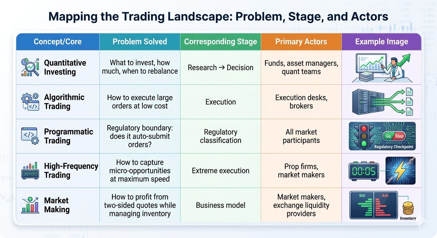
These five concepts deserve to be dissected one by one, because confusing them is one of the main ways outsiders misunderstand quant.
Quantitative Investing: The Research and Decision Brain
The core of quantitative investing is using systematic, data-driven methods to study asset pricing, build portfolios, and manage risk. It answers: what to hold, how much to hold, and when to rebalance. It corresponds to the “research → decision” stage of the trading process.
A quant researcher does not sit in front of candlestick charts waiting for intuition. They stare at tables.
They might ask: “Do low P/E stocks systematically outperform high P/E stocks over the next month?” Then they translate that into a statistical test: after removing survivorship bias, neutralizing by sector, and accounting for size, is this premium still significant? If so, does it persist out-of-sample? Under what regimes does it fail?
After that, they blend this factor with others (momentum, quality, low volatility) and run them through a portfolio optimizer to answer: under sector deviation constraints (say, within ±2%), market-cap neutrality, and turnover capped at 30%, how should capital be allocated to maximize information ratio?
The moat here is: depth of research, data quality, factor discovery, and the systematic nature of portfolio construction. The output is not a “buy signal”; it is a fully specified portfolio.
Algorithmic Trading: The Hands and Feet of Execution
Algorithmic trading uses algorithms to determine how orders are executed. It solves: “How do I trade a large order without blowing out the price?” It sits at the “execution” stage of the process.
Imagine a pension fund that needs to sell 1 million shares of a moderately liquid stock. If it simply dumps a 1-million-share market order, it will smash through the order book, and the average sell price will be far below the current quote. That is market impact.
The job of the execution algorithm is to break this parent order into thousands of child orders and feed them into the market over hours like water seeping into sand, so that the average fill is as close as possible to the volume-weighted average price (VWAP) or the time-weighted average price (TWAP) over that window.
It does not care whether the stock goes up or down tomorrow. It only cares: can I finish this trade within the specified time window, at minimal impact?
ESMA explicitly includes order slicing as algorithmic trading. The moat is: deep understanding of microstructure, low-latency execution systems, and stable connectivity to exchanges and dark pools. Its value is “saved transaction cost.”
Program Trading
Program trading is not a strategy; it is a regulatory category.
The CSRC defines it as “automatically generating or submitting trading instructions via computer programs”. This is a wide net. It covers:
Full CTA strategies that use code to generate and execute orders.
Pure execution algos that only slice orders.
High-frequency order behavior.
The point is not to describe a strategy, but to mark regulatory boundaries: if you auto-submit, you need to report; if you are high-frequency, you may face tiered fees and tighter anomaly monitoring. Program trading is a compliance concept, not a competitive edge.
High-Frequency Trading: The Extremes of Speed and Microstructure
HFT is an extreme subset of algorithmic trading. Its defining features are ultra-short holding periods (milliseconds to seconds), very high order and cancel rates, and extreme sensitivity to latency.
Picture two co-located servers in an exchange data center, connected by the shortest fiber. One runs an order-book analytics model, parsing real-time feed at microsecond granularity and computing shifts in buying and selling pressure across dozens of price levels. When a sudden buildup of bids appears at a particular level, the system jumps in before competitors, captures the micro-move, holds for a few seconds, and liquidates.
Each trade earns a fraction of a cent. The profits come from astronomical repetition. The moat is speed, system quality, queue position, hardware (FPGA), and real-time risk — a capital-intensive arms race.
Market Making: A Two-Sided Quoting Business Model
Market making is the business of continuously posting both buy and sell quotes, earning the spread, and managing the inventory risk this creates.
Market makers almost always use high-frequency technology to update quotes and hedge risks quickly. But not all HFT is market making.
A typical market-making trade looks like this: post a bid at 99.50 and an offer at 100.50. If both sides get hit, you earn 1 unit of spread. If only one side trades, you now have inventory risk and must hedge or adjust quotes.
The moat is quoting strategy, inventory models, capital strength, exchange relationships, and very fast risk systems. The profit comes from liquidity provision, not price forecasting.
You can summarize the relationship like this:
Quant investing decides what to own and how much.
Algorithmic trading decides how to send orders.
HFT is “sending orders using the fastest possible algorithms.”
Market making is a spread-earning business built on two-sided quoting.
Program trading is the regulatory basket holding all of the above auto-order activity.
Two concrete business chains make this clearer.
Public mutual fund enhanced product: the quant team builds multi-factor models and chooses which stocks to overweight or underweight. The optimizer outputs the target holdings. Execution algos then take these targets and use something like VWAP to finish the trades at low cost. Under regulations, the algorithmic execution is program trading and must be reported.
Options market maker: the quoting engine uses a volatility surface model to compute a theoretical price of, say, 102. It posts offers at 103 and bids at 101, and keeps both sides live. The generation and adjustment of these quotes is fully automated. The high-frequency component is the part that updates quotes in microseconds to reflect new information. This entire chain is also program trading in the regulatory sense.
So What Is This Article Actually Trying to Answer?
Not: “How to use Python to write a strategy in three days.”
But more fundamentally:
Where did quantitative trading come from?
What branches has it grown into today?
Who is doing what, internationally?
What actually makes money?
Why do so many beautiful backtests die in live trading?
And what is the most useful way a normal person should think about quant?
We can put the core conclusion up front:
Quantitative trading is not magic. It is the act of putting trading under repeated interrogation by data, rules, costs, risk, and time.
Where It Came From
Quantitative trading was not invented in the Internet era. The intellectual lineage is long.
In the mid-twentieth century, Harry Markowitz’s portfolio theory made the “risk–return tradeoff” into a formally computable problem. William Sharpe’s CAPM further systematized portfolio risk and asset pricing. Nobel citations explicitly state that Markowitz’s theory of portfolio selection laid the foundation for subsequent work in financial economics, and Sharpe’s CAPM built upon Markowitz’s work.
Another strand comes from asset pricing and market efficiency. Eugene Fama received the Nobel Prize for empirical work on market efficiency and asset pricing. The Kenneth French Data Library institutionalized the Fama-French factor framework, which remains one of the most widely used factor databases in both academia and industry globally. The language of “value, size, profitability, investment, momentum” that circulates today is not trade jargon improvised on social media — it is the distilled output of decades of academic research and industrial investment.
This lineage directly shaped multi-factor investing, index enhancement, risk models, and style rotation. When people say “value, size, profitability, investment, momentum” today, they are not using random trader slang — they are speaking a language jointly shaped by long-run academic research and industrial-scale investing.
To be precise, this is a conceptual summary, not a linear historical timeline. From Markowitz to CAPM to Fama-French, then to option pricing and electronic trading — these are multiple research lines evolving in parallel and intersecting. But this conceptual routing helps build a coherent mental map.
Then comes derivatives pricing and risk management. The 1997 Nobel citation states directly that the methods of Black, Scholes, and Merton opened the way for valuing options and, more broadly, derivatives, and enabled more efficient risk management. Modern options quant, volatility trading, market making, and Greeks-based risk control all live in this lineage. You cannot talk seriously about options quant without talking about implied volatility, Gamma, Vega, volatility surfaces, and margin.
Electronic trading pushed everything up a tier. Regulatory and infrastructure evolution turned algos from “research ideas” into actual execution engines.
ESMA’s algorithmic trading rules require that firms have robust systems with thresholds and limits to prevent erroneous orders from disrupting markets.
The US SEC’s Market Access Rule (Rule 15c3-5) requires brokers with exchange access to implement risk controls and supervisory procedures.
At this point, quant becomes not just research but systems engineering. Beyond the model, you now need risk limits, price limits, duplicate-order prevention, logging, rollbacks, disaster recovery, permissions, and full audit trails.
Modern quant then took another step: from daily and intraday bars plus fundamental and factor data, into limit order books, market microstructure, alternative data, and machine learning.
DeepLOB studies how to use deep learning to read order books.
MLOFI studies how multi-level order-flow imbalances explain mid-price moves.
The CFA Institute’s AI and Big Data handbook puts ML, text, alt data, and microstructure execution into one industry framework.
These studies show that order books, ML, and alternative data can be treated seriously. They do not imply that a normal person with a single model can obtain stable profits.
Which is to say: when people say “quant” today, they are not talking about a single tree; they are talking about an entire forest. Some branches connect to asset management, some to exchange microstructure, some to data science and engineering.
The Seven Branches, and What Each Actually Earns
The most useful way to decompose quantitative trading is not by difficulty, but by what it earns, what data it depends on, and what infrastructure it requires.
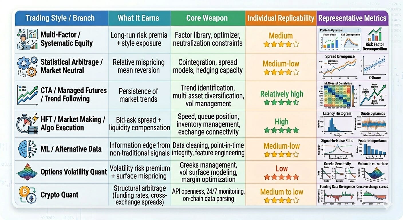
Multi-Factor and Systematic Equity Selection
The most common branch is multi-factor and systematic stock selection.
MSCI is explicit: factor investing is about identifying the risk and return drivers of a portfolio within a consistent framework. Kenneth French’s five-factor page spells out exactly how those factors are constructed.
AQR’s Equity Market Neutral Fund states openly that it pursues absolute return independent of market direction by running long–short portfolios across hundreds of companies and diversified signals. AQR’s Style Premia Alternative Fund goes further, extending value, momentum, carry, and defensive style premia across equities, bonds, rates, commodities, and currencies.
This is not “guess which stock goes up tomorrow.” It is about turning cross-sectional characteristics into something that can be combined, neutralized, and constrained.
Operationally, the logic is straightforward but not easy: historically, some firm characteristics — cheapness, strong profitability, recent outperformance, low volatility, etc. — have shown statistical relationships with future returns. The implementation is:
Quantify those characteristics across the stock universe (e.g., value as 1/P/E, momentum as 12‑month return excluding the most recent month).
Use an optimizer to combine them into a portfolio, subject to sector neutrality, market-cap neutrality, and risk exposure constraints.
On the institutional side, AQR and Dimensional Fund Advisors are the canonical examples. On the China side, most index enhancement products, systematic equity funds, and many private strategies (whether price-volume or fundamental factors) speak the same underlying language.
Fama & French (1993) and their 2015 five-factor model are the bedrock here. Harvey, Liu, and Zhu’s paper on the “factor zoo” is mandatory reading: they document about 316 published factors in their sample and show why traditional significance thresholds (t > 2.0) are no longer acceptable under multiple testing. Bali, Engle, and Murray’s Empirical Asset Pricing gives a very usable operational framework, and the Kenneth French Data Library is where you go to test whether your factor construction works out of sample.
But there’s a harsher truth you have to accept: the factors you can see in public databases are mostly survivors. By the time an individual investor recreates a historically beautiful factor from the French Library, that factor’s golden age is usually already over. The real fight happens in the “dark forest” period before academic publication and industrial rollout.
Institutions are no longer playing the simple five-factor game. They are:
Timing factors dynamically.
Or hunting micro-level signals that are extremely tightly reasoned and not yet published.
You also have to stay clear-eyed: factors can fail, and they can get crowded. From 2018 to 2020, value factors in US equities significantly trailed growth, and funds with persistent value exposure took real pain. Whether that period represents a temporary compression of the value risk premium or a structural failure is still debated. The partial comeback of value factors in 2022–2024, especially outside the US, complicates the story. It’s not honest to cite that episode as clean proof that “value is dead.”
Statistical Arbitrage and Market Neutral
The second branch is statistical arbitrage and market-neutral strategies.
These strategies don’t bet on the overall direction of the market. They bet on relationships: spread reversion, relative value, portfolio mispricing, style dislocations.
The form most people see is not the cointegration formula in a textbook, but fund labels like “market neutral,” “absolute return,” or “style premia.”
AQR’s public product descriptions and Winton’s materials both stress low correlation, absolute return, and diversification — not “99% win-rate” stories. Whether they make money or not has nothing to do with slogans and everything to do with this question: Can you consistently capture a recurring but decaying statistical relationship after all costs?
Compared to multi-factor, the emphasis shifts. Stat arb focuses more on relative relationships among assets:
The classic pattern is pairs trading: two highly correlated stocks, where the spread relative to their historical mean blows out; you go long the cheap one, short the rich one, and bet on mean reversion.
More complex structures use cointegration and PCA to identify long-run equilibrium relationships across multiple assets and trade deviations from that equilibrium.
Market neutral is often the packaging: you go long and short so that your portfolio’s beta to the market is near zero, and you earn the relative strength between your longs and shorts.
Gatev, Goetzmann, and Rouwenhorst (2006) is the canonical paper on pairs trading. The important footnote: subsequent studies, like Do & Faff (2010) across global markets and Broussard & Vaihekoski (2012) for Finnish equities, document that the excess returns in the original paper decayed sharply after publication. You should not assume the original performance numbers still hold. Avellaneda & Lee (2010) show a PCA-based approach; Vidyamurthy’s Pairs Trading is a focused monograph on this direction.
But statistical relationships can break. The 2007 “quant quake” was the textbook disaster: large market-neutral portfolios with highly similar holdings, one side forced to deleverage, cascading unwinds, and suddenly assets that historically had little to do with each other start moving together violently. The lesson is clear:
The biggest risk in statistical arbitrage is not that the model is “wrong.” It is that too many people are using similar models on the same relationships.
CTA, Managed Futures, and Systematic Trend
The third branch is CTA/managed futures/systematic trend following.
Strictly speaking:
CTA is a registration category in US futures regulation.
Managed futures is a strategy category.
Trend following is the most common and representative, but not the only, implementation of managed futures.
The NFA defines a CTA as someone who, for compensation, advises about the value or advisability of trading futures, options, retail forex, or swaps. AQR describes managed futures as a systematic strategy that goes long and short global, highly liquid futures and forwards across equities, rates, currencies, and commodities. Winton’s UCITS documents make it clear: trend is often the core, but other diversifying signals get added to survive non-trending regimes.
The strengths of CTA and managed futures are obvious: transparent logic, a long history, and relatively straightforward to wrap into regulated products. The downsides are equally transparent: long periods of chop and drawdowns. It is not a machine that “makes money every month.”
The branch logic is the most blunt of all: the core bet is “trends continue.” When prices rise, go long; when they fall, go short; when a threshold is breached, stop out. Under the hood, you usually see moving-average crossovers, channel breakouts (e.g., Donchian channels), and momentum indices across equity indices, government bonds, commodities, and FX, all diversified.
The more uncorrelated markets you include, the harder it is for any single market to kill the portfolio.
Moskowitz, Ooi, and Pedersen (2012) give the canonical “Time Series Momentum” paper.
Hurst, Ooi, and Pedersen’s 2017 Journal of Portfolio Management article uses around 130 years of data to show long-term effectiveness, but they explicitly note the limitations of early data quality and coverage. “130 years of evidence” should be read as “within the scope of available data,” not as a divine guarantee.
Entry-level reading: Clenow’s Stocks on the Move and Covel’s Trend Following. Institutional examples: Winton and Man AHL. In China’s futures markets, trend strategies have been around for a long time and have relatively low barriers to entry.
But CTA’s main enemy is not trend reversals; it is extended non-trending chop. From roughly 2009 to 2013, many CTAs suffered: global markets oscillated without a clear direction, and trend signals were eroded repeatedly. The most common way individual CTA developers die is not because their logic is wrong, but because they cannot psychologically endure months of grind and shut down the strategy right before a major move.
CTA return distributions are extremely skewed: most profits come from a small number of big trends. The rest of the time is mild bleeding or small gains. After 6–12 months of drawdown, conviction collapses, you pull the plug — and the market promptly delivers a decade-best trend without you. That’s not a coding problem; it’s a human problem under long-term pressure.
Modern institutional CTA is also far beyond pure price momentum. Firms like Winton and Man AHL already weave alternative data into their trend engines — satellite imagery, shipping flows — to gauge the sustainability of commodity trends. This layer is almost impossible for an individual to replicate.
I adopted the strategy for Gold only with some refinement, and I’ll explain it further in the next chapter. One of my reasons is cost efficiency. For the machine learning approach I originally considered, the required data—whether it’s tick‑level order book history, alternative data streams, or a particular vendor’s curated dataset—costs more than $2,000 per year just for the base subscription, without even counting add‑on services. That fixed cost is not viable on my current capital, and unless I can secure enough funding, this path is simply out of my options. I suspect many undercapitalised retail quants face the same barrier: it’s not that machine learning itself is unaffordable, but that acquiring the right data to make a specific ML strategy work can be prohibitively expensive. DeepSeek’s CEO adopted ML strategy.
HFT, Market Making, and Algorithmic Execution
The fourth branch is HFT, market making, and execution algos — the part that outsiders most often lump together.
Regulators treat HFT as a demanding subset of algorithmic trading, characterized by:
Ultra-low latency.
Heavy order-book interaction.
Queue-position sensitivity.
Very high message rates.
Real-time automated risk control.
Market making is about continuously posting two-sided quotes, earning the bid–ask spread, and managing inventory risk. Execution algorithms answer “how do I trade this big order,” not “where is the market going.”
VWAP and TWAP are classic examples: they exist to reduce market impact for large trades, not to predict returns.
ESMA’s materials explicitly state that slicing large orders to optimize execution counts as algorithmic trading. Citadel Securities, Optiver, and Virtu all describe themselves using market maker, liquidity, two-sided prices, and technology on their websites. Jane Street calls itself a research-driven trading firm and emphasizes capital, global reach, technology, expertise, and quantitative trading.
The moat here is rarely “a magical factor.” It’s speed, systems, risk controls, exchange connectivity, quoting capacity, and capital efficiency.
That’s why a retail trader buying a fancy backtesting framework is not “getting closer to Jane Street.”
A market maker’s core business is to continuously quote bids and offers, buy at bid and sell at ask, and earn the spread. HFT’s moat is almost entirely infrastructure:
Better feed decoding.
Lower network latency.
Better queue positions on exchanges.
More accurate microstructure models.
Real-time risk and kill-switches.
Citadel Securities, Optiver, and Virtu sell “liquidity infrastructure,” not magic prediction engines. VWAP/TWAP and similar algos are engineering products to break large orders into smaller ones and minimize cost. They are decoupled from the investment thesis.
For individuals, this branch is nearly impossible to copy — not because the strategies are conceptually hard, but because the infrastructure bill is ruinous: co-location, low-latency NICs, dedicated fiber, full-depth real-time feeds, and the software stack to handle all that.
Even many institutional asset managers can no longer credibly enter this game at the cutting edge. From FPGAs to ASICs, from microwave towers to the shortest submarine-cable routes across oceans, the limiting factor is now physics: the speed of light.
And this field is going through a regime shift: scale is beating speed.
Historically, “being fast” was the core HFT moat. Now, according to public reports, Citadel Securities handles a huge chunk of US retail equity order flow, not because it is strictly faster than everyone, but because it can internalize flow at scale — match buyers and sellers inside its own system rather than sending everything to exchanges. For these firms, speed is still important, but the information edge and inventory efficiency that come from flow scale overshadow the pure latency race.
Citadel Securities and Virtu make money from liquidity and spreads. They are not playing the same game as traditional hedge funds like AQR or D.E. Shaw. The former are “off-balance-sheet liquidity infrastructure for exchanges”; the latter are “correctors of pricing errors.”
Machine Learning, Alternative Data, and Microstructure Modeling
The fifth branch is machine learning, alternative data, and microstructure modeling.
The CFA Institute’s reports on AI and big data in investing say the quiet part out loud: ML’s appeal is better risk-adjusted returns, but financial data is unusually hostile — noisy, non-stationary, sample-poor, with strong feedback effects.
Harvey, Arnott, and Markowitz’s work on backtesting protocols in the ML era emphasizes the same point: ML in finance does not automatically solve the problems that dog traditional quant models. Overfitting, poor experimental design, and data limitations still dominate.
At the same time, Nasdaq’s and QuantConnect’s alternative data pages show just how far the input universe has expanded: credit card data, geolocation, medical claims, supply chains, text, sentiment, web activity — all are in play.
The question, however, is not “Is this data cool?” but:
Is this signal point-in-time (actually available at the time), compliant, tradable, and scalable?
AI will keep pushing deeper into quant research, coding, data processing, text analysis, monitoring, and risk. But the more realistic first-order effect is productivity, not magically turning a retail user’s model into stable alpha.
This branch is more “tool-upgrade” than a standalone profit source. ML can be used:
To read order books (CNNs on LOB data).
To parse earnings calls (NLP).
To synthesize factors (gradient boosting, etc.).
Alternative data can include satellite imagery, anonymized card transactions, social media sentiment, and logistics flows.
CFA materials and Harvey et al. keep hammering the same warning: the signal-to-noise ratio in finance is extremely low; data is scarce, non-stationary, and subject to feedback. ML’s pattern-finding power becomes a double-edged sword — it becomes easier to find good-looking but fake patterns.
This is exactly where individuals are most likely to hallucinate “shortcut to the big leagues,” because Python and ML libraries are free. In reality, the kill shot is almost always:
Data compliance.
Point-in-time integrity.
Self-scraped social sentiment data usually has severe survivorship bias and timestamp problems. The institutions paying millions for anonymized credit card flows, or satellite data, spend at least half of that just on cleaning and aligning it to backtests. Without that data foundation, your deep learning model is just drawing portraits of noise.
And institutions have dedicated data compliance teams. Individuals scraping or buying certain alt data can step on regulatory landmines without even realizing it.
Options Volatility Quant
The sixth branch is options volatility quant.
If stock multi-factor work is about cross-section, options quant is about surfaces — volatility and risk transfer.
The OIC and CME’s educational materials both emphasize implied volatility, historical volatility, Gamma, and Vega as core objects of pricing and risk. Cboe’s VIX methodology is industrialized “reverse-engineering expected volatility from options prices.”
In other words, many options strategies are not earning from directional calls. They’re earning:
Volatility risk premia.
Term structure.
Skew.
Hedging errors.
Liquidity compensation.
These strategies often show high win rates and small day-to-day drawdowns. The problem is tail risk. When the rare-but-destructive event arrives, the losses can be instantaneous.
This is the “picking up coins in front of a steamroller” structure. As long as markets are calm, you collect a premium steadily. When something like March 2020’s liquidity crisis or an August 2024 VIX spike comes along, the explosion in implied volatility can crack your margins in a single session, wiping out years of accumulated profits. In real stress, dynamic hedging often fails — you simply cannot adjust quickly enough before the account is gone.
The fundamental difference from other branches is:
You are trading volatility, not price direction.
The core logic: options prices embed expectations of future volatility (implied volatility); historical volatility is realized past volatility; the gap between them is the volatility risk premium. Many strategies revolve around selling overpriced volatility and buying underpriced volatility, hedging Delta to strip out directional exposure and leave a relatively pure volatility exposure.
In practice, this is brutally dependent on:
Real-time Greeks (Delta, Gamma, Vega, Theta).
Volatility surface modeling.
Margin management.
The VIX index is just one industrialized product that reverse-engineers the market’s “fear level” from options prices.
Crypto Quant
The seventh branch is crypto quant.
Crypto markets made many individuals feel “institutional-grade” for the first time, because:
APIs are open.
Markets run 24/7.
Spot, perpetual futures, options, funding rates, and on-chain data are all easily accessible.
Binance, OKX, and Bybit all provide public order book, trade, and funding rate APIs. Coin Metrics sells on-chain and digital-asset data products.
But openness is not the same as “easy.”
You get easier data access and full exposure to:
Exchange risk.
API rate limits and behavior changes.
Matching engine changes.
Liquidity migration.
Forced liquidations and auto-deleveraging.
Regulatory shocks.
Crypto quant looks democratized on the surface. In reality, it just moved the gate from “you can’t get data” to:
“You’ve got the data, but can you actually process and survive it?”
Structurally, crypto has some unique features:
24/7 trading.
Funding rate mechanisms in perpetual futures (periodic transfers between longs and shorts).
Transparent on-chain data.
Frequent cross-exchange spreads.
Common strategies include:
Funding-rate arbitrage (long spot, short perp to collect high positive funding).
Cross-exchange arbitrage.
On-chain MEV (extracting value from transaction ordering).
Momentum/trend following on crypto assets.
The visible barrier is low — APIs are open, data is rich, and instruments are many. The hidden costs are high:
Exchange default or fraud risk.
API rate limits and rule changes.
Liquidity is shifting rapidly between venues.
Catastrophic liquidations and auto-deleveraging in extreme moves.
More subtly, some exchanges implement preferential matching rules for retail flow. This can create a gap between “visible liquidity in the API” and “actually tradeable liquidity.” Backtests are generally less reliable than in traditional markets: a perfect equity curve on one exchange and one period often collapses when moved to a different venue or time window.
If this framework resonated with you:
👏 Clap this article if you believe macro analysis should be quantifiable, not subjective.
🔁 Repost it to help another trader break free from the “overriding the algorithm” trap.
💬 Comment with the one macro event you think most traders consistently misread—let’s make it systematic.
This tells people exactly what to do and why it matters to the community.